
 Image: Rob Schultz
Excel’s Text functions are a major time saver if your job entails managing massive data, especially data that’s imported from other sources. Fortunately, all ASCII data is easily imported, but the format of that imported data can vary drastically from one source to another.
For example, fields may be delimited, such as with tabs, spaces, commas, or periods. Aany other characters are all preferable to spaces. That’s because spaces not only exist in between fields, they also separate words within the fields, which makes sorting out the fields a real challenge. That’s where the following Text functions are very helpful.
A. Use the SUBSTITUTE function to replace one string of text with another
Function syntax: The syntax (or sentence structure) of the SUBSTITUTE function is this:
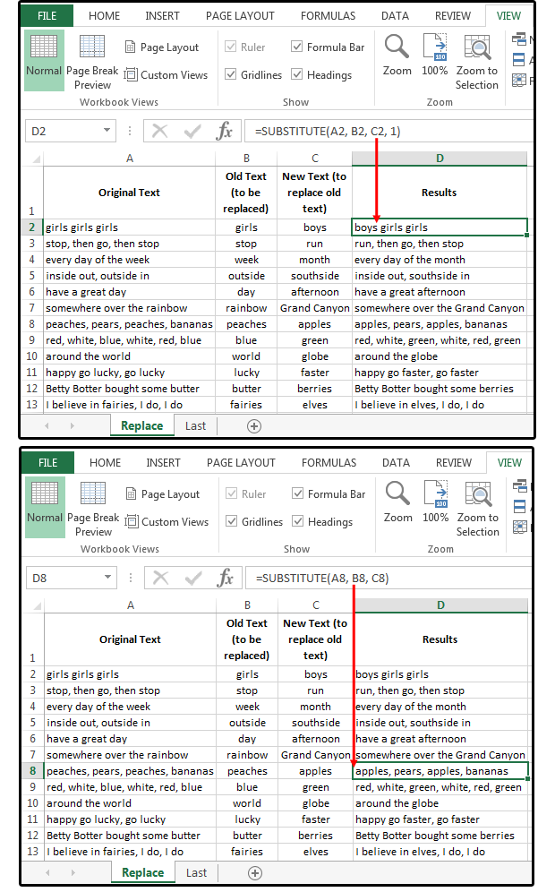
=SUBSTITUTE(text, old text, new text, [Instance Num]).
Note: If you don’t specify an Instance Num, every occurrence of the Old Text is changed to the New Text. If you specify the Instance Num, only that occurrence of the Old Text is replaced. For example, entering the number ‘1’ means you want to change only the first occurrence of that word in the string.
1. Enter some phrases in column A (from A2 through A13).
2. Enter the word or phrase you want changed in column B.
3. Enter the word or phrase you want to replace the old text with in column C.
4. Enter the following formula in cells D2 through D7 (or half the database): =SUBSTITUTE(A2, B2,C2,1)
This changes/replaces only the first occurrence of the Old Text to New Text.
5. Next, enter this formula in the remaining cells (in our case, D8 through D13): =SUBSTITUTE(A2, B2,C2). This changes/replaces all occurrences of the Old Text to New Text.
Note: This function is case-sensitive, so if your results aren’t working, change the text to all the same case.
 PC World / JD Sartain
01 Use the SUBSTITUTE function to replace one string of text with another
B. Extract the last word in a string of text using TRIM, RIGHT, & SUBSTITUTE
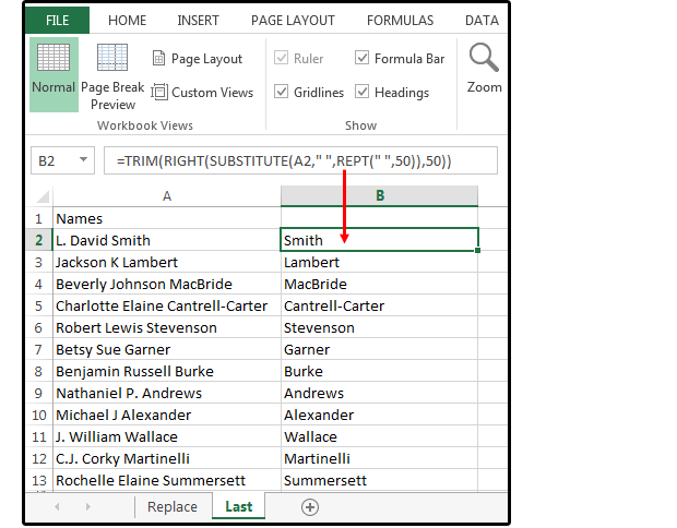
For this example, the object is to extract the last word—that is, the last name, from a string of text (the full names of a list of clients).
1. Enter some names in column A: first, last, and middle names or initials.
2. Enter this formula in B2: =TRIM(RIGHT(SUBSTITUTE(A2,” “,REPT(“ “,50)),50)).
3. Copy the formula from B2, down to B3 through B1000 (or the end of your database). For this example, we’re assuming your database has 1,000 records.
4. This formula works because the SUBSTITUTE function locates all the spaces in the string of text, and then replaces each single space with 50 spaces. The RIGHT function removes 50 characters (from right to left), and the TRIM function deletes all the excess leading spaces leaving just the single, last word. If you have longer strings of text, try substituting 100 or more for the 50 values in the above formula.
 PC World / JD Sartain
Extract the last word in a string of text
Further Excel training
If you want to deepen your Excel mastery, a number of online courses exist to expand your knowledge. Here are our top picks to start with:
Coursera – Excel Skills for Business: Essentials
EDX – Analyzing and Visualizing Data with Excel
Lynda.com – Excel: Scenario Planning and Analysis
Udacity – Excel Fundamentals
C. Extract the first word/name in a string of text using LEFT & SEARCH
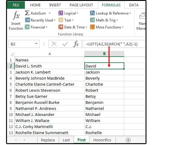
This formula works when you need to separate the first name from the middle and last name of a list of clients.
1. Enter some names in column A (or use the same names from the previous exercise).
2. Enter this formula in B2 through B1000: =LEFT(A2,SEARCH(“ “,A2)-1) to extract the first name of each client into a separate column.
 PC World / JD Sartain
Extract the first word/name in a string of text
D. Extract everything except the first word in a string of text using TRIM, RIGHT, REPT, & SUBSTITUTE
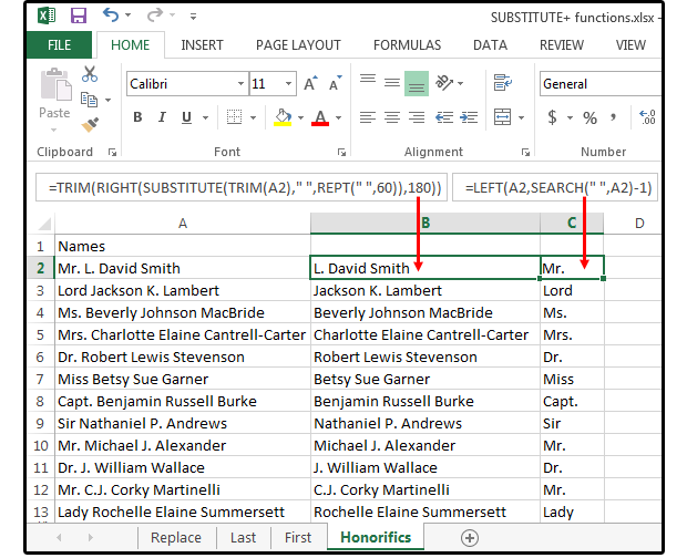
The purpose of this exercise is to remove the honorifics from a list of client names. These clients are providing confidential survey information, so the company does not want the titles and salutations of each individual to influence the surveyors.
1. Enter some more names in column A (or use the same names from the previous exercise). Enter some honorifics before each name; e.g., Mr., Miss, Ms, Mrs. , Dr., Sir, Lord, Lady, Capt., etc.
2. Enter this formula in B2 through B1000: =TRIM(RIGHT(SUBSTITUTE(TRIM(A2),” “,REPT(“ “,60)),180)) to extract the full names of all the clients minus the honorifics.
3. And, if you wanted to extract the honorifics (for some reason), enter this formula in C2 through C1000: =LEFT(A2,SEARCH(“ “,A2)-1).
 PC World / JD Sartain
Extract everything EXCEPT the first word in a string of text
E. Extract names from email addresses using LEFT, FIND, & SUBSTITUTE
The worst job of the day is to spend hours manually retyping client names or domain names from email addresses, especially when the list is over 5,000 names. Use the following formulas to complete this task in minutes.
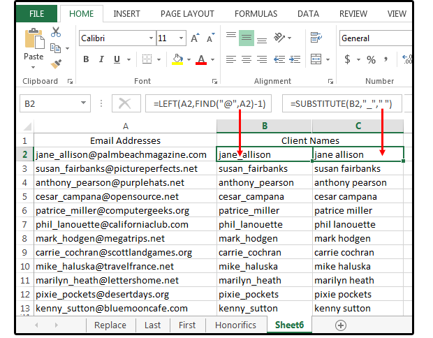
1. Enter some email addresses in column A.
2. Enter this formula in B2 through B5000: =LEFT(A2,FIND(“@”,a2)-1) to extract the full names of all the clients.
3. Enter this formula in C2 through C5000 to remove the underscore between the first and last name: =SUBSTITUTE(B2,” “,”_”).
4. Move to cell F2. Select Formulas > Text > . Type C2 in the Text field box on the Functions Arguments dialog screen, or click cell C2, and then click OK. This formula converts the names to Proper Case (that is, first letter of the first and last name capitalized, all other letters in lowercase).
5. Copy the formula in F2 to F3 through F5000 and press Enter.
 PC World / JD Sartain
Extract names from email addresses
G. Extract domains from email addresses using TRIM, LEFT, SUBSTITUTE, MID, FIND, LEN, & REPT
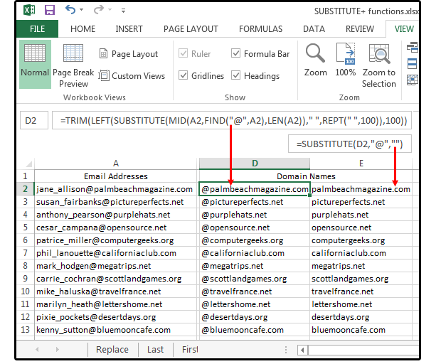
1. Enter this formula in D2 through D5000 to extract the domain names from the email addresses:
=TRIM(LEFT(SUBSTITUTE(MID(A2,FIND(“@”,A2),LEN(A2)),” “,REPT(“ “,100)),100))
2. And last, enter this formula in E2 through E5000 to remove the @ signs from the extracted domain names: =SUBSTITUTE(D2,”@”,””).
 PC World / JD Sartain
Extract domains from email addresses


