
 Image: Rob Schultz
Excel Conditional Formatting already lets you format cells based on the value of those cells or the value of the formulas in those cells (see our conditional formatting tutorial for more details). Now we’ll show how you can customize these features so you (and others) can quickly scan your spreadsheet and determine at a glance what the data means based on the way each column, row, cell, or range is formatted.
Here’s how to find the customization options. In any spreadsheet, choose Home > Conditional Formatting > New Rule. The New Formatting Rule dialog window opens.
Notice the first panel: Select a Rule Type. We’ll go through the options in turn:
Format all cells based on their valuesFormat only cells that containFormat only top or bottom ranked valuesFormat only values that are above or below averageFormat only unique or duplicate valuesUse a formula to determine which cells to format
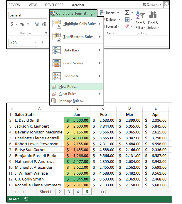 PC World / JD Sartain
Create new rules for conditional formatting.
For this tutorial we’ve created a simple spreadsheet showing the sales figures for a team over the months of January through April.
Format all cells based on their values: Color Scales
1. Highlight column B (Jan Sales Totals) and choose Home > Conditional Formatting > New Rule.
2. Select the first option, Format all cells based on their values.
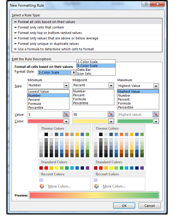
3. In the lower panel, Edit the Rule Description, there are four options under Format All Cells Based on Their Values.
4. Under Format Style, select 2-Color Scale or 3-Color Scale. You can customize the Minimum and Maximum or Minimum, Midpoint, and Maximum values, respectively.
5. Under Type > Minimum, Midpoint, Maximum, select Lowest, Highest, Number, Percent, Formula, or Percentile based on how you’d like to see the numbers in your database grouped.
6. Choose a value for the Number, Percent, Formula, or Percentile.
7. Choose the Colors, then click OK.
 PC World / JD Sartain
Format cells based on values and a color scale
Format all cells based on their values: Data Bars
1. Highlight column C (Feb Sales Totals) and choose Home > Conditional Formatting > New Rule.
2. Select the first option, Format all cells based on their values, again.
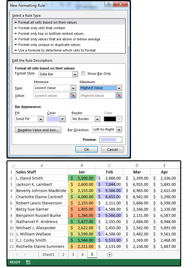
3. In the bottom panel, Edit the Rule Description, there are four options under Format All Cells Based on Their Values.
4. Select Format Stylle: Data Bar.
5. Scroll through the options in the bottom panel and choose the Minimum and Maximum Type and Value.
6. In the Bar Appearance section, select the Fill (Solid or Gradient); the Color; the Border and Border Color; and the Bar Direction (Context, Left-to-Right, or Right-to-Left).
7. Last, enter the Negative Value and Axis (if applicable).
Note: Data bars are a useful way of seeing trends in data, and negative value data bars help analyze trends when negative values are involved.
 PC World / JD Sartain
Format cells based on values: Data Bars
Format all cells based on their values: Icon Sets
1. Highlight column D (Mar Sales Totals) and choose Home > Conditional Formatting > New Rule.
2. Select the first option, Format all cells based on their values.
3. In the bottom panel, Edit the Rule Description, under Format All Cells Based on Their Values, choose Format Style: Icon Sets.
4. Click the arrow beside Icon Style and choose a style from the drop-down list.
Under the next section, Display each icon according to these rules:
5. Use the default icon or select a custom icon from the drop-down list.
6. Enter the value of the first icon, then enter the value type (Number, Percent, Formula, Percentile). Remember to click the down arrow on the left side of the Value field box and choose one of the greater/less than or equal-to symbols.
7. Enter the remaining Values and Types, then click OK when finished.
 PC World / JD Sartain
Format cells based on their values using Icon Sets
Format only cells that contain
1. Highlight column E and choose Home > Conditional Formatting > New Rule.
2. Select the second option: Format only cells that contain.
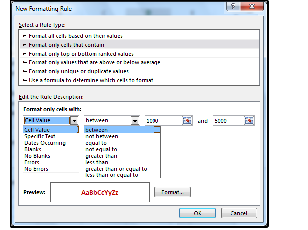
3. In the Edit the Rule Description panel, select an option from the first field drop-down list: Cell Value, Specific Text, Dates Occurring, Blanks, No Blanks, Errors, No Errors. For this exercise, choose Cell Value.
4. From the second field, choose a condition such as Between, Not Between, Equal To, Not Equal To, Greater Than, Less Than, Greater Than or Equal To, or Less Than or Equal To. For this exercise, choose Between.
5. In the next two fields, enter the Between this and Between that values. For example, enter between 1000 and 5000.
 PC World / JD Sartain
Format only cells that contain specific values.
6. Click the Format button and choose a Font, Font Color, Font Style, Border, and Fill Colors, Effects, and Patterns. In this case, choose the Bold attribute and the Color purple.
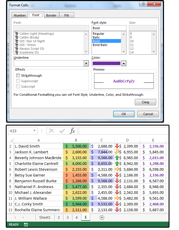 PC World / JD Sartain
Format Font, Colors, Style, Border, and Fill
Format only top or bottom ranked values
1. Highlight column B and choose Home > Conditional Formatting > New Rule.
2. Select the third option: Format only top or bottom ranked values.
3. In the Edit the Rule Description panel—under Format Values that Rank in the: select Top or Bottom and a number, such as Top 10, or a percentage, such as Top 40%.
4. In our example, we formatted the matched values in orange italics. Note that only four numbers in column B meet this criteria.
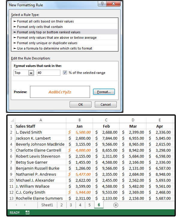 PC World / JD Sartain
Format only top- or bottom-ranked values.
Format only values that are above or below average
1. Highlight column C and choose Home > Conditional Formatting > New Rule.
2. Select the fourth option: Format only values that are above or below average.
3. In the Edit the Rule Description panel, under Format Values That Are, choose the average for the selected range.
4. Click the down arrow beside the list box and select an option from the list, such as Above, Below, Equal or Above, Equal or Below and more. For this example, select Above.
5. Click the Format button to select your Custom Formats, including Font, Border Style & Color; Fill/Shade Design, Color, Pattern, and more. In this case, we chose Font: Bold red. Next, click OK. Note that all the numbers in column C that are above average are now displayed in bold red.
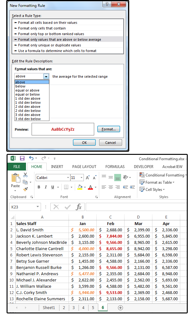 PC World / JD Sartain
08 Format only values that are above or below average
Format only unique or duplicate values
1. Highlight column D and choose Home > Conditional Formatting > New Rule.
2. Select the fifth option: Format only unique or duplicate values.
3. In the Edit the Rule Description panel under Format All Values in the Selected Range, click the down arrow beside the list box and select Duplicate or Unique from the list.
4. Click the Format button to select your Custom Formats. In this case, we chose a Regular purple font (that is, not Italics or Bold) with purple dotted lines framed around all the duplicate values. Next, click OK. Note that all the Duplicate numbers in column D are now displayed in regular purple within a purple dotted frame.
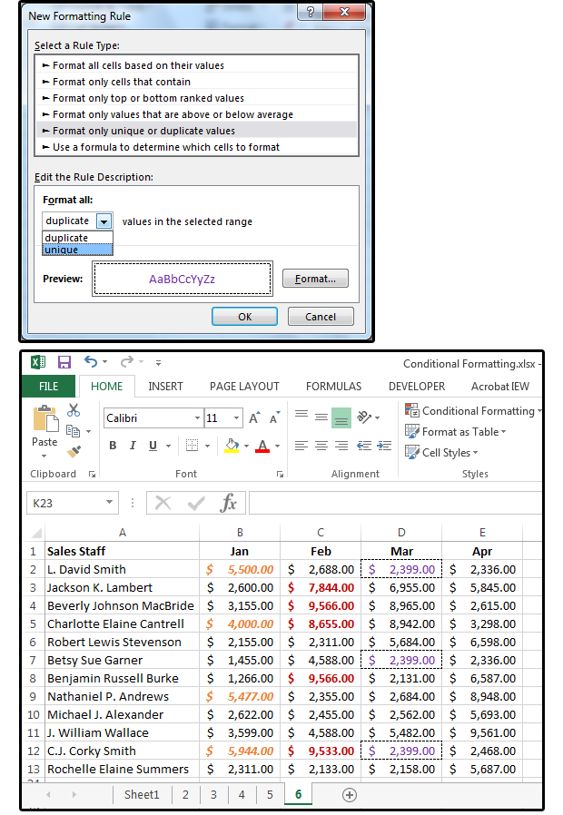 PC World / JD Sartain
09 Format only unique or duplicate values
Use a formula to determine which cells to format
1. Highlight column E and choose Home > Conditional Formatting > New Rule.
2. Select the sixth option: Use a formula to determine which cells to format.
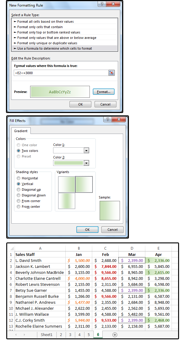
3. In the Edit the Rule Description panel under Format Values Where This Formula Is True, enter a formula in the field box that highlights the values you want selected. In this case, we entered +E2<=3000.
4. Click the Format button to select your Custom Formats. Under Font, choose Bold, dark green. Under Fill, choose Fill Effects.
6. Choose Gradient, then select a Gradient Style.
7. Choose a Gradient Color (Two Colors, Color 1 = white and Color 2 = light green).
8. Then click OK. Note that all the values in column E that are less than or equal to 3000 are now displayed in a dark-green font with a green-to-white gradient fill/shade.
 PC World / JD Sartain
Use a formula to determine which cells to format
Excel offers thousands of ways to custom-format the data in your spreadsheets. Play around with the options and find out what works best for you.


